Oslo wavy workshop 2024
The following examples are tailored to the wavy Workshop. This workshop will focus on some simple examples that can be used as python code snippets in your workflow.
0. checklist wavy installation
did you add your wavy root directory to $PYTHONPATH?
is wavy activated? (conda activate wavy)
1. wavy config files
For this workshop you will need the following config files:
satellite_cfg.yaml.default   insitu_cfg.yaml.default
model_cfg.yaml.default
Create a new project directory. Establish an .env file such that wavy knows where to find the config files it should use. This could look like:
:~$ mkdir ws24_wavy
:~$ cd ws24_wavy
:~/ws24_wavy$ touch .env
:~/ws24_wavy$ mkdir config
Now copy the needed config default files from wavy/wavy/config to this directory and remove the suffix .default. The result would look like:
:~/ws24_wavy/config$ ls
insitu_cfg.yaml     satellite_cfg.yaml    model_cfg.yaml
This is the structure of your project directory:
:~/ws24_wavy$ ls -la
total 16
drwxrwxr-x  3 patrikb patrikb 4096 Nov 14 09:04 .
drwx------ 79 patrikb patrikb 4096 Nov 14 09:06 ..
drwxrwxr-x  2 patrikb patrikb 4096 Nov 14 09:10 config
-rwxr-xr-x  1 patrikb patrikb   44 Nov 14 09:04 .env
Where your .env-file needs to point to this config folder like in the following example for my username patrikb:
:~/ws24_wavy$ cat .env
WAVY_CONFIG=/home/patrikb/ws24_wavy/config/
WAVY_DIR=/home/patrikb/wavy/
Finally, the same .env file has to be copied to the wavy root directory, ~/wavy.
2. Download L3 satellite altimetry data
L3 satellite data is obtained from Copernicus with the product identifier WAVE_GLO_WAV_L3_SWH_NRT_OBSERVATIONS_014_001. User credentials are required for this task. So before you can start you have to get a Copernicus account (free of costs). Prepare access to Copernicus products. Enter your account credentials into the .netrc-file. The .netrc should be located in your home not being too permissive like:
:~$ ls -lh .netrc
-rwx------ 1 patrikb patrikb 675 Oct 19 07:54 .netrc
Your .netrc should look something like:
machine nrt.cmems-du.eu login {USER} password {PASSWORD}
Adjust the satellite config file called satellite_cfg.yaml. Remember, this is the file you copied to ~/ws24_wavy/config. It should include the following section and could look like:
--- # specifications for satellite missions

cmems_L3_NRT:
    # mandatory
    name:
        s3a: s3a
        s3b: s3b
        c2: c2
        j3: j3
        h2b: h2b
        al: al
        cfo: cfo
        s6a: s6a
    # mandatory when downloading
    # where to store downloaded data
    download:
        ftp: # downloading method
            src_tmplt: "/Core/\
                        WAVE_GLO_PHY_SWH_L3_NRT_014_001/\
                        cmems_obs-wave_glo_phy-swh_nrt_name-l3_PT1S/\
                        %Y/%m/"
            trgt_tmplt: /home/patrikb/tmp_altimeter/L3/name/%Y/%m
            path_date_incr_unit: 'm'
            path_date_incr: 1
            search_str: '%Y%m%dT'
            strsub: ['name']
            server: "nrt.cmems-du.eu"
    # optional: where to read from
    #           can be defined directly when calling wavy
    wavy_input:
        src_tmplt: /home/patrikb/tmp_altimeter/L3/name/%Y/%m
        fl_tmplt: "varalias_name_region_\
                        %Y%m%d%H%M%S_%Y%m%d%H%M%S.nc"
        strsub: ['name']
        path_date_incr_unit: 'm'
        path_date_incr: 1
    # optional: where to write to
    #           can be defined directly when calling wavy
    wavy_output:
        trgt_tmplt: /home/patrikb/tmp_altimeter/L3/name/%Y/%m
        fl_tmplt: "varalias_name_region_\
                        %Y%m%d%H%M%S_%Y%m%d%H%M%S.nc"
        strsub: ['varalias','name','region']
        file_date_incr: m
    # optional, if not defined the class default is used
    reader: read_local_ncfiles
    collector: get_remote_files_cmems
    # optional, needs to be defined if not cf and in variable_info.yaml
    vardef:
        Hs: VAVH
        U: WIND_SPEED
    coords:
    # optional, info that can be used by class functions
    misc:
        processing_level:
        provider:
        obs_type:
    # optional, to ease grouping
    tags:
Amend the path_template line and correct it according to the directory you want to store satellite data. For my directory the line is:
cmems_L3:
   ftp:
      trgt_tmplt: /home/patrikb/tmp_altimeter/L3/name
You can proceed now and download L3 data using the wavyDownload.py script:
$ cd ~/wavy/apps/standalone
To get help check …
$ ./wavyDownload.py --help
… then download some satellite altimeter data:
$ ./wavyDownload.py --nID cmems_L3_NRT --name s3a --sd 2023020100 --ed 2023020200 --nproc 4
-nproc 4 means 4 simultaneous downloads. This can be adjusted according to resources and needs. You can find the downloaded files in your chosen download directory. Now download some other dates for later use.
3. Read satellite data
Once the satellite data is downloaded one can access and read the data for further use with wavy. Let’s have a look at some examples in a python script.
In python L3-data can be read by importing the satellite_class, choosing a region of interest, the variable of interest (Hs or U), the satellite mission, which product should be used, and whether a time window should be used as well as a start and possibly an end date. This could look like:
>>> from wavy.satellite_module import satellite_class as sc
>>> # settings
>>> region = 'global'
>>> varalias = 'Hs'  # default
>>> name = 's3a'
>>> nID = 'cmems_L3_NRT'
>>> twin = 30  # default
>>> sd = "2023-2-1 11"  # can also be datetime object
>>> ed = "2023-2-1 12"  # not necessary if twin is specified
>>> # retrieval
>>> sco = sc(sd=sd, ed=ed, region=region, nID=nID, name=name)
>>> sco = sco.populate()
This would result in a satellite_class object and the following output message:
# -----
 ### Read files and populate satellite_class object
 ## Find and list files ...
path is None -> checking config file
Object is iterable
8 valid files found
source template: /home/patrikb/tmp_altimeter/L3/name/%Y/%m

Checking variables..
 Get filevarname for
stdvarname: sea_surface_wave_significant_height
varalias: Hs
 !!! standard_name:  sea_surface_wave_significant_height  is not unique !!!
The following variables have the same standard_name:
 ['VAVH', 'VAVH_UNFILTERED']
 Searching *_cfg.yaml config file for definition
 Variable defined in *_cfg.yaml is:
Hs = VAVH

Choosing reader..
Chosen reader: satellite_readers.read_local_ncfiles

Reading..
Reading 10 chunks of files with chunk size 1
Total of 8 files
100%|██████████████████████████████████████████████████████████| 9/9 [00:00<00:00, 56.61it/s]
 changing variables to aliases
 Get filevarname for
stdvarname: sea_surface_wave_significant_height
varalias: Hs
 !!! standard_name:  sea_surface_wave_significant_height  is not unique !!!
The following variables have the same standard_name:
 ['VAVH', 'VAVH_UNFILTERED']
 Searching *_cfg.yaml config file for definition
 Variable defined in *_cfg.yaml is:
Hs = VAVH
   VAVH is alreade named correctly and therefore not adjusted
 Get filevarname for
stdvarname: time
varalias: time
 Get filevarname for
stdvarname: longitude
varalias: lons
   lons is alreade named correctly and therefore not adjusted
 Get filevarname for
stdvarname: latitude
varalias: lats
   lats is alreade named correctly and therefore not adjusted
 enforcing lon max min = -180/180

 ## Summary:
5211 footprints retrieved.
Time used for retrieving data:
0.17 seconds

 ### satellite_class object populated ###
# -----
Note that we first initialized the satellite_class object with the following line:
>>> sco = sc(sd=sd, ed=ed, region=region, nID=nID, name=name)
And we then populated it with data using the populate method:
>>> sco = sco.populate()
If you have not downloaded satellite data with wavyDownload.py, you can also initialize a satellite object with the same parameters you would use for the import, and use the download method. Note that you still need to configure the satellite_cfg.yaml accordingly:
>>> sco = sc(sd=sd, ed=ed, region=region, nID=nID, name=name)
>>> sco.download()
Another option is to give the path directly to the download function:
>>> sco.download(path='.....')
Investigating the satellite_object you will find something like:
>>> sco.
sco.edate             sco.processing_level  sco.twin
sco.get_item_child(   sco.product           sco.units
sco.get_item_parent(  sco.provider          sco.varalias
sco.label             sco.quicklook(        sco.varname
sco.mission           sco.region            sco.vars
sco.obstype           sco.sdate             sco.write_to_nc(
sco.path_local        sco.stdvarname        sco.write_to_pickle(
With the retrieved variables in sco.vars:
>>> sco.vars
<xarray.Dataset>
Dimensions:  (time: 5211)
Coordinates:
  * time     (time) datetime64[ns] 2023-02-01T10:33:27 ... 2023-02-01T12:26:16
Data variables:
    Hs       (time) float32 1.145 0.999 0.826 0.763 ... 1.368 1.379 1.38 1.384
    lons     (time) float64 -149.9 -150.0 -150.2 -150.4 ... 150.0 150.0 150.0
    lats     (time) float64 -76.35 -76.31 -76.26 -76.22 ... -36.99 -36.93 -36.87
Attributes:
    title:    wavy dataset
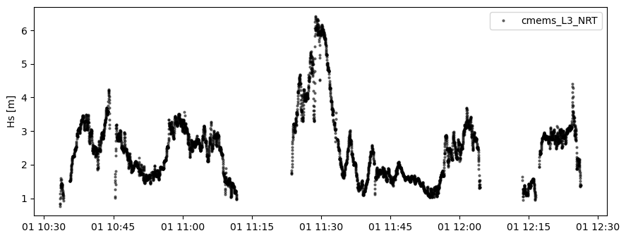
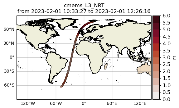
Using the quicklook function you can quickly visualize the data you have retrieved:
>>> sco.quicklook(ts=True) # for time series
>>> sco.quicklook(m=True) # for a map
>>> sco.quicklook(a=True) # for all
|
|
Exercise:
Define your own region in region_cfg.yaml and retrieve satellite data for this region.
4. access/read in-situ data
In-situ observations can also be imported using the insitu_module module. You can add new sources of in-situ data using the insitu_cfg.yaml file, just like in the satellite_cfg.yaml.
>>> from wavy.insitu_module import insitu_class as ic
>>> varalias = 'Hs'
>>> sd = "2023-12-2 00"
>>> ed = "2023-12-5 00"
>>> nID = 'D_Breisundet_wave'
>>> sensor = 'wavescan'
>>> ico = ic(nID=nID, sd=sd, ed=ed, varalias=varalias, name=sensor)
>>> ico = ico.populate()
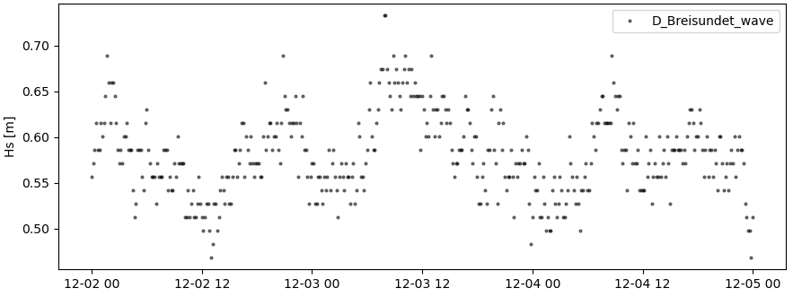
You can have a look at the obtained time series:
>>> sco.quicklook(ts=True)
5. access/read model data
Model output can be accessed and read using the model_module module. The model_module config file model_cfg.yaml needs adjustments if you want to include a model that is not present as default.
You can then import model data as follows:
>>> from wavy.model_module import model_class as mc
>>> nID = 'ww3_4km'  # default
>>> varalias = 'Hs'  # default
>>> sd = "2023-6-1"
>>> ed = "2023-6-1 01"
>>> mco = mc(nID=nID, sd=sd).populate()  # one time slice
>>> mco_p = mc(nID=nID, sd=sd, ed=ed).populate()  # time period
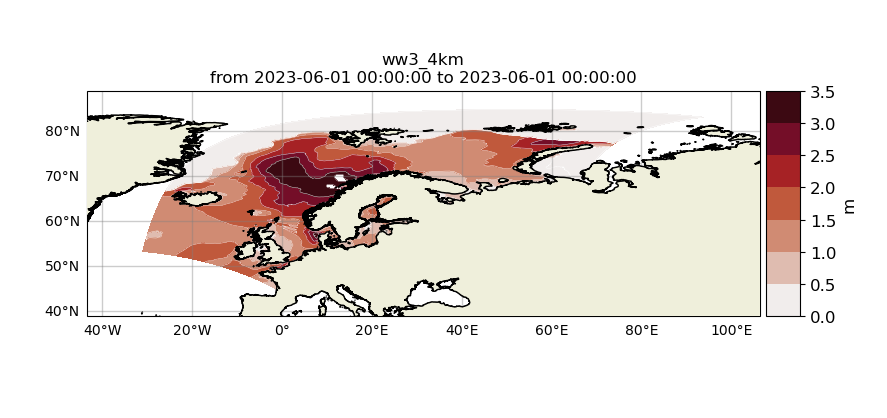
And again it is possible to visualize the data:
>>> sco.quicklook(m=True)
6. Collocating model and observations
One main focus of wavy is to ease the collocation of observations and numerical wave models for the purpose of model validation. If you have available the necessary satellite data and model data you can proceed with collocation:
Collocation of satellite and wave model
>>> from wavy.satellite_module import satellite_class as sc
>>> from wavy.collocation_module import collocation_class as cc
>>> sd = "2023-2-1 11"
>>> ed = "2023-2-1 11"
>>> name = 's3a'
>>> varalias = 'Hs'
>>> twin = 29  # in minutes
>>> nID = 'cmems_L3_NRT'
>>> model = 'ww3_4km'

>>> # initialize satellite_object
>>> sco = sc(sd=sd, ed=ed, nID=nID, name=name,
>>>          varalias=varalias, twin=twin)

>>> # read data
>>> sco = sco.populate()

>>> # crop to region
>>> sco = sco.crop_to_region(model)

>>> # collocate
>>> cco = cc(oco=sco, model=model, leadtime='best', distlim=6)
distlim is the distance limit for collocation in km and date_incr is the time step increase in hours. One can also add a keyword for the collocation time window. The default is +-30min which is equivalent to adding twin=30. In this case ERA only had 6h time steps which makes it a bit more unlikely that satellite crossings and model time steps coincide. Increasing twin helps, however, it means we assume quasi-stationarity for this time period.
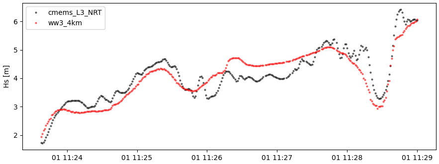
Using the quicklook function again (cco.quicklook(a=True)) will enable three plots this time, a time series plot (ts=True), a map plot (m=True), and a scatter plot (sc=True).
>>> cco.quicklook(ts=True)
7. Validate the collocated time series
Having collocated a quick validation can be performed using the validationmod. validation_metrics.yaml can be adjusted.
>>> val_dict = cco.validate_collocated_values()

# ---
Validation stats
# ---
Correlation Coefficient: 0.89
Mean Absolute Difference: 0.35
Root Mean Squared Difference: 0.41
Normalized Root Mean Squared Difference: 0.10
Debiased Root Mean Squared Difference: 0.41
Bias: -0.05
Normalized Bias: -0.01
Scatter Index: 10.03
Model Activity Ratio: 0.98
Mean of Model: 4.02
Mean of Observations: 4.08
Number of Collocated Values: 317
The entire validation dictionary will then be in val_dict.
8. Regridding data
Once satellite observations are retrieved or even collocated model data are available wavy can process and display this data in custom grids for your region of interest.
Gridding of satellite data
Let us try it with satellite data first. Note that here we import the files using path parameter in sco.populate(). This allows to import all files from a given directory. Again, the format of the file must be defined in satellite_cfg.yml.
>>> from wavy.satellite_module import satellite_class as sc

>>> path_to_files = '/home/patrikb/wavy/tests/data/L3/s3a/'
>>> sd = '2022-2-1'
>>> ed = '2022-2-2'
>>> region = 'NordicSeas'
>>> name = 's3a'
>>> nID = 'cmems_L3_NRT'
>>> sco = sc(sd=sd, ed=ed, region=region, nID=nID, name=name)
>>> sco = sco.populate(path=path_to_files)
Now the gridder can be applied as follows:
>>> from wavy.gridder_module import gridder_class as gc
>>> from wavy.grid_stats import apply_metric
>>> bb = (-20, 20, 60, 80) # lonmin,lonmax,latmin,latmax
>>> res = (5, 5) # lon/lat
>>> gco = gc(lons=sco.vars.lons.squeeze().values.ravel(),
>>> lats=sco.vars.lats.squeeze().values.ravel(),
>>> values=sco.vars.Hs.squeeze().values.ravel(),
>>> bb=bb, res=res,
>>> varalias=sco.varalias,
>>> units=sco.units,
>>> sdate=sco.vars.time,
>>> edate=sco.vars.time)
>>> gridvar, lon_grid, lat_grid = apply_metric(gco=gco)
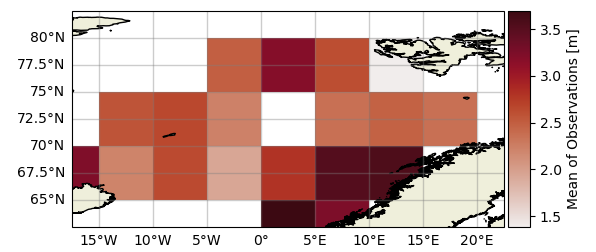
>>> gco.quicklook(val_grid=gridvar,
>>> lon_grid=lon_grid,
>>> lat_grid=lat_grid,
>>> metric='mor', land_mask_resolution='i',
>>> mask_metric_llim=1,
>>> title='')
Information of the grid and the values from observations and model can also be obtained directly from the gridder_class object:
>>> ovals, mvals, Midx = gco.get_obs_grid_idx()
Gridding of collocated data
It is also possible to grid the collocated data.
>>> from wavy.collocation_module import collocation_class as cc
>>> # collocate
>>> cco = cc(model='ww3_4km', oco=sco, distlim=6, leadtime='best', date_incr=1)
>>> # reduce region to part of model domain for better visual
>>> bb = (-20, 20, 50, 80) # lonmin,lonmax,latmin,latmax
>>> res = (5, 5) # lon/lat
>>> gco = gc(cco=cco, bb=bb, res=res)
>>> var_gridded_dict, lon_grid, lat_grid = apply_metric(gco=gco)
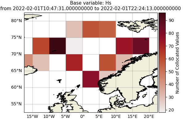
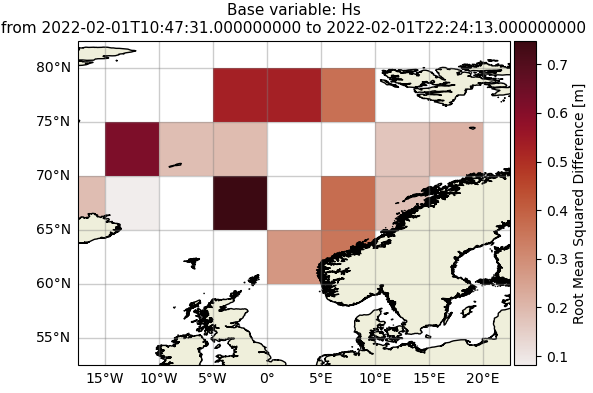
>>> # plot all validation metrics on grid
>>> gco.quicklook(val_grid=var_gridded_dict, lon_grid=lon_grid, lat_grid=lat_grid, metric='all')
|
|
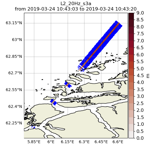
9. Applying filters
Finally, it is possible to apply some filters to the data. Let us try it on some L2 satellite data already included in the package.
>>> from wavy.satellite_module import satellite_class as sc
>>> path_to_files= '/home/patrikb/wavy/tests/data/CCIv3_20Hz/'
>>> sd = '2019-3-24 10'
>>> ed = '2019-3-24 11'
>>> region = 'Sulafj'
>>> sco = sc(sd=sd, ed=ed,
>>>          nID='L2_20Hz_s3a', name='s3a',
>>>          region=region)
>>> sco = sco.populate(path=path_to_files)
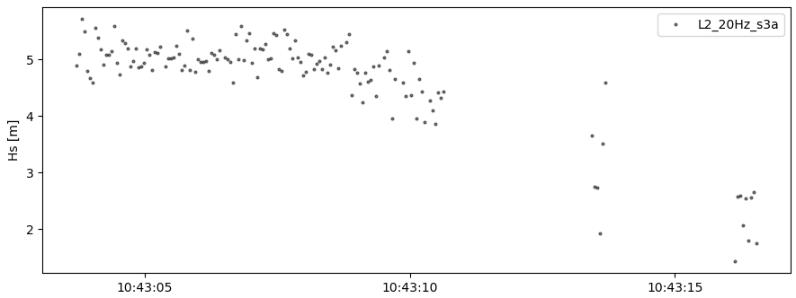
You can have a first look at the data:
>>> sco.quicklook(a=True, land_mask_resolution='f')
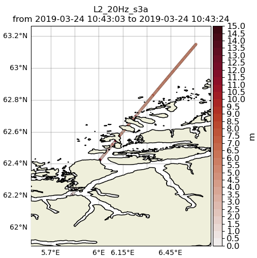
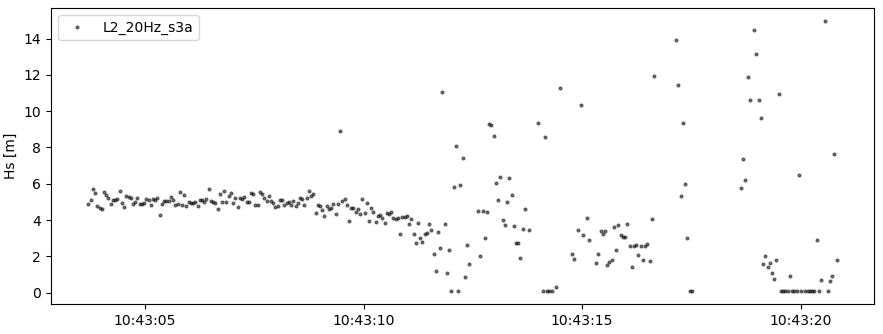
There could be some land interactions with the satellite track. It is possible to filter it using sco.filter_landMask() function. Additionnally points closer than a certain distance to the coast can be defined using sco.filter_distance_to_coast() with llim argument. If specifics (range gate resolution and height over ground) about the satellite intsrument are known one can compute a possible foot print land interaction based on the size of the pulse limited footprint size byt adding .filter_footprint_land_interaction(). Finally, values under threshold (resp. over) can also be discarder using the sco.apply_limits() method with llim argument (resp. ulim).
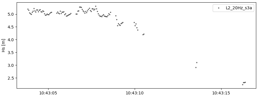
The corresponding code is the following:
>>> sco_filter = sco.filter_landMask()\
...                 .filter_distance_to_coast(llim=650)\
...                 .filter_footprint_land_interaction()\
...                 .apply_limits(llim=0.1)
This can be plotted by:
>>> sco.quicklook(a=True, land_mask_resolution='f')
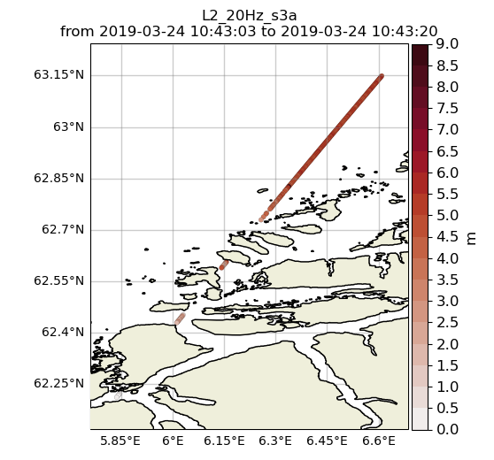
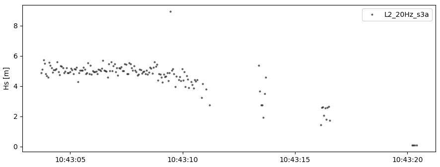
In order to show the computed x-track pulse-limited footprint size one can add:
>>> sco_filter.quicklook(a=True, land_mask_resolution='f', plot_xtrack_pulse_limited_fpr=True)
Some additional despiking method can be applied with sco.despike_blockStd().
>>> sco_despike = sco_filter.despike_blockStd(slider=20, sigma=2, chunk_min=5, sampling_rate_Hz=20)
Another operation you can perform is smoothing the time serie, using a running mean with the sco.filter_runmean method:
>>> sco_smooth = sco_despike.filter_runmean(window=5, chunk_min=5, sampling_rate_Hz=20)
10. Saving data to netcdf
It is possible to save the data from the different wavy objects to .nc files. If we take again the first example we used for the satellite data:
>>> from wavy.satellite_module import satellite_class as sc
>>> # settings
>>> region = 'global'
>>> varalias = 'Hs'  # default
>>> name = 's3a'
>>> nID = 'cmems_L3_NRT'
>>> twin = 30  # default
>>> sd = "2023-2-1 11"  # can also be datetime object
>>> ed = "2023-2-1 12"  # not necessary if twin is specified
>>> # retrieval
>>> sco = sc(sd=sd, ed=ed, region=region, nID=nID, name=name)
>>> sco = sco.populate()
Then we can save the data contained in sco.vars as follows:
>>> sco.vars.to_netcdf('/home/patrikb/ws24_wavy/test_dump.nc')
This way, you can directly reimport the data by initializing a new satellite_class object and populate it giving the path to the netcdf file created earlier in the sco.populate() method using wavy_path argument as follows:
>>> from wavy.satellite_module import satellite_class as sc
>>> # settings
>>> region = 'global'
>>> varalias = 'Hs'  # default
>>> name = 's3a'
>>> nID = 'cmems_L3_NRT'
>>> twin = 30  # default
>>> sd = "2023-2-1 11"  # can also be datetime object
>>> ed = "2023-2-1 12"  # not necessary if twin is specified
>>> # retrieval
>>> sco = sc(sd=sd, ed=ed, region=region, nID=nID, name=name)
>>> sco = sco.populate(wavy_path='/home/patrikb/ws24_wavy/test_dump.nc')
Note that this works with insitu_class and model_class object as well.