Read in-situ observations (netcdf/thredds, FROST API)

Currently 3 datasources can be accessed: nc-files, thredds-server, and FROST API. Edit the insity_specs.yaml file in your config folder and adjust the directories.

make a FROST call

For a FROST call wavy uses MET Norways FROST API v1. A FROST call would be similar compared to the satellite and model retrieval, here illustrated for the Draugen platform:

>>> from wavy.insitu_module import insitu_class as ic

>>> varalias = 'Hs' # default
>>> sd = "2021-8-2 01"
>>> ed = "2021-8-3 00"
>>> nID = 'draugen'
>>> sensor = 'MKIIIradar_1'
>>> ico = ic(nID=nID, sd=sd, ed=ed, varalias=varalias, name=sensor)
>>> ico = ico.populate()

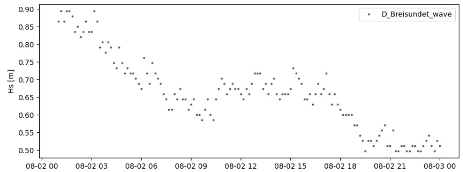
read .nc-files

>>> from wavy.insitu_module import insitu_class as ic

>>> varalias = 'Hs'
>>> sd = "2021-8-2 01"
>>> ed = "2021-8-3 00"
>>> nID = 'D_Breisundet_wave'
>>> sensor = 'wavescan'
>>> ico = ic(nID=nID, sd=sd, ed=ed, varalias=varalias, name=sensor)
>>> ico = ico.populate()

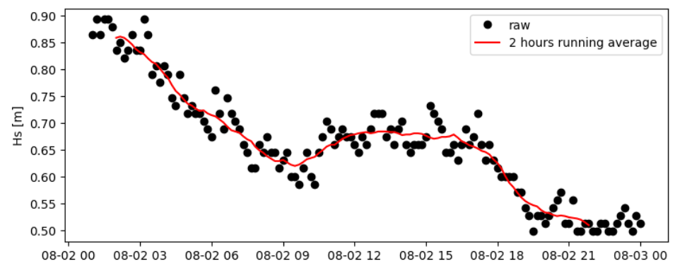
Then you can smooth the obtained time series with a running mean, specifying the number of observations used and the sampling rate of the measurements:

>>> # running mean filter
>>> ico_rm = ico.filter_runmean(window=13, sampling_rate_Hz=1/600)

Now, let’s check how this could look like:

>>> import matplotlib.pyplot as plt
>>> fig = plt.figure(figsize=(9,3.5))
>>> ax = fig.add_subplot(111)
>>> ax.plot(ico.vars['time'],ico.vars[varalias],'ko',label='raw')
>>> ax.plot(ico_rm.vars['time'],ico_rm.vars[varalias],'r-',label='2 hours running average')
>>> plt.legend(loc='upper right')
>>> plt.ylabel('Hs [m]')
>>> plt.show()

Again, for the insitu class there is also a quicklook function available:

>>> ico.quicklook(ts=True)