Vietnam Validation Workshop 2022 #2
Note
The codes used for this workshop are from an older version of wavy. It can be adapted with the newest version of the package, however you can still find the version used for this workshop on github.
The following examples are tailored to the 4. wavy Vietnam Validation Workshop and second workshop in 2022. While the first part in 2022 was in spring and dedicated to trajectories, this workshop will focus on some simple examples that can be used as python code snippets in your workflow.
1. wavy config files
For this workshop you will need the following config files:
collocation_specs.yaml.default  region_specs.yaml.default
satellite_specs.yaml.default    quicklook_specs.yaml.default
model_specs.yaml.default        validation_specs.yaml.default
Create a new project directory. Establish an .env file such that wavy knows where to find the config files it should use. This could look like:
:~$ mkdir ws22_wavy
:~/ws22_wavy$ mkdir config
Now copy the needed config default files from wavy/wavy/config to this directory and remove the suffix .default. The result would look like:
:~/ws22_wavy/config$ ls
collocation_specs.yaml  region_specs.yaml
model_specs.yaml        satellite_specs.yaml
quicklook_specs.yaml    validation_specs.yaml
This is the structure of your project directory:
:~/ws22_wavy$ ls -la
total 16
drwxrwxr-x  3 patrikb patrikb 4096 Nov 14 09:04 .
drwx------ 79 patrikb patrikb 4096 Nov 14 09:06 ..
drwxrwxr-x  2 patrikb patrikb 4096 Nov 14 09:10 config
-rwxr-xr-x  1 patrikb patrikb   44 Nov 14 09:04 .env
Where your .env-file needs to point to this config folder like in the following example for my username patrikb:
:~/ws22_wavy$ cat .env
WAVY_CONFIG=/home/patrikb/ws22_wavy/config/
The main changes that will occur in the config files during this workshop are:
adjusting the path
adding your model
2. Download L3 satellite altimetry data
L3 satellite data is obtained from Copernicus with the product identifier WAVE_GLO_WAV_L3_SWH_NRT_OBSERVATIONS_014_001. User credentials are required for this task. So before you can start you have to get a Copernicus account (free of costs). Prepare access to Copernicus products. Enter your account credentials into the .netrc-file. The .netrc should be located in your home not being too permissive like:
:~$ ls -lh .netrc
-rwx------ 1 patrikb patrikb 675 Oct 19 07:54 .netrc
Your .netrc should look something like:
machine nrt.cmems-du.eu login {USER} password {PASSWORD}
Adjust the satellite config file called satellite_specs.yaml. Remember, this is the file you copied to ~/ws22_wavy/config. It should include the following section and could look like:
--- # specifications for satellite missions

cmems_L3_NRT:
     mission:
         s3a: s3a
         s3b: s3b
         c2: c2
         al: al
         j3: j3
         h2b: h2b
         cfo: cfo
     dst:
         path_template: /home/patrikb/tmp_altimeter/L3/mission
         file_template: "varalias_mission_region_\
                         %Y%m%d%H%M%S_%Y%m%d%H%M%S.nc"
         strsub: ['varalias','mission','region']
         file_date_incr: m
     src:
         path_template: "/Core/\
                 WAVE_GLO_WAV_L3_SWH_NRT_OBSERVATIONS_014_001/\
                 dataset-wav-alti-l3-swh-rt-global-mission/%Y/%m/"
         server: "nrt.cmems-du.eu"
         strsub: ['mission']
     misc:
     vardef: # varalias: varname
         Hs: VAVH
         U: WIND_SPEED
     processing_level: L3
     provider: cmems
Amend the path_template line and correct it according to the directory you want to store satellite data. For my directory the line is:
cmems_L3:
   dst:
      path_template: /home/patrikb/tmp_altimeter/L3/mission
You can proceed now and download L3 data using the wavyDownload.py script:
$ cd ~/wavy/apps/standalone
To get help check …
$ ./wavyDownload.py -h
… then download some satellite altimeter data:
$ ./wavyDownload.py -sat s3a -sd 2020110100 -ed 2020111000 -product cmems_L3_NRT -nproc 4
-nproc 4 means 4 simultaneous downloads. This can be adjusted according to resources and needs. You can find the downloaded files in your chosen download directory. Now download some other dates for later use.
$ ./wavyDownload.py -sat s3a -sd 2021112600 -ed 2021120300 -product cmems_L3_NRT -nproc 4
3. Read satellite data
Once the satellite data is downloaded one can access and read the data for further use with wavy. Let’s have a look at some examples in a python script.
In python L3-data can be read by importing the satellite_class, choosing a region of interest, the variable of interest (Hs or U), the satellite mission, which product should be used, and whether a time window should be used as well as a start and possibly an end date. This could look like:
>>> from wavy.satmod import satellite_class as sc
>>> region = 'NorwegianSea'
>>> varalias = 'Hs' # default
>>> mission = 's3a' # default
>>> product = 'cmems_L3_NRT' # default
>>> twin = 30 # default
>>> sd = "2020-11-1" # can also be datetime object
>>> ed = "2020-11-10" # not necessary if twin is specified
>>> sco = sc(sdate=sd,edate=ed,region=region)
This would result in a satellite_class object and the following output message:
# -----
 ### Initializing satellite_class object ###

Requested time frame: 2020-11-01 00:00:00 - 2020-11-10 00:00:00
Chosen time window is: 30 min
No download initialized, checking local files

 ## Find files ...
path_local is None -> checking config file
/home/patrikb/tmp_altimeter/L3/s3a/2020/10
/home/patrikb/tmp_altimeter/L3/s3a/2020/11
89 valid files found

 ## Read files ...
Get filevarname for
stdvarname: sea_surface_wave_significant_height
varalias: Hs
!!! standard_name:  sea_surface_wave_significant_height  is not unique !!!
The following variables have the same standard_name:
['VAVH', 'VAVH_UNFILTERED']
Searching *_specs.yaml config file for definition
Variable defined in *_specs.yaml is:
Hs = VAVH
100%|██████████████████████████████████████████| 89/89 [00:00<00:00, 214.94it/s]
Concatenate ...
... done concatenating
Total:  400391  footprints found
Apply region mask
Specified region: NorwegianSea
 --> Bounded by polygon:
lons: [5.1, -0.8, -6.6, -9.6, -8.6, -7.5, 1.7, 8.5, 7.2, 16.8, 18.7, 22.6, 18.4, 14.7, 11.7, 5.1]
lats: [62.1, 62.3, 63.2, 64.7, 68.5, 71.1, 72.6, 74.0, 76.9, 76.3, 74.5, 70.2, 68.3, 66.0, 64.1, 62.1]
Values found for chosen region and time frame.
Region mask applied
For chosen region and time:  3551 footprints found

 ## Summary:
3551 footprints retrieved.
Time used for retrieving satellite data: 0.64 seconds

 ### Satellite object initialized ###
# -----
Investigating the satellite_object you will find something like:
>>> sco.
sco.edate             sco.processing_level  sco.twin
sco.get_item_child(   sco.product           sco.units
sco.get_item_parent(  sco.provider          sco.varalias
sco.label             sco.quicklook(        sco.varname
sco.mission           sco.region            sco.vars
sco.obstype           sco.sdate             sco.write_to_nc(
sco.path_local        sco.stdvarname        sco.write_to_pickle(
With the retrieved variables in sco.vars:
>>> sco.vars.keys()
dict_keys(['sea_surface_wave_significant_height', 'time', 'time_unit', 'latitude', 'longitude', 'datetime', 'meta'])
Using the quicklook function you can quickly visualize the data you have retrieved:
>>> sco.quicklook(ts=True) # for time series
>>> sco.quicklook(m=True) # for a map
>>> sco.quicklook(a=True) # for all
You can dump your data using sco.write_to_nc or sco.write_to_pickle like:
>>> sco.write_to_nc('/home/patrikb/ws22_wavy/data/testfile.nc')
Dump data to netCDF4 file
Dump data to file:  /home/patrikb/ws22_wavy/data/testfile.nc
Exercise:
Define your own region in region_specs.yaml and retrieve satellite data for this region.
4. access/read model data
Model output can be accessed and read using the modelmod module. The modelmod config file model_specs.yaml needs adjustments if you want to include a model that is not present as default. Given that the model output file you would like to read follows the cf-conventions and standard_names are unique, the minimum information you have to provide are usually:
modelname:
    path_template:
    file_template:
    init_times: []
    init_step:
Often there are ambiguities due to the multiple usage of standard_names. Any such problem can be solved here in the config-file by adding the specified variable name like:
vardef:
    Hs: VHM0
    time: time
    lons: lon
    lats: lat
The variable aliases (left hand side) need to be specified in the variable_info.yaml. Basic variables are already defined. Adding your model output files to wavy means to add something like:
ecwam_vietnam:
    vardef:
        Hs: significant_wave_height
        time: time
        lons: longitude
        lats: latitude
    path_template: "/home/patrikb/Documents/Vietnam/%Y/"
    file_template: "vietnam_wave_%Y%m%d_%H.nc"
    init_times: [0,12]
    init_step: 12
    date_incr: 3
    proj4: "+proj=longlat +a=6367470 +e=0 +no_defs"
    grid_date: 2021-11-26 00:00:00

ecifs_vietnam:
    vardef:
        ux: u10m
        vy: v10m
        time: time
        lons: lon
        lats: lat
    path_template: "/home/patrikb/Documents/Vietnam/%Y/"
    file_template: "ECIFS%Y%m%d%H.nc"
    init_times: [0,12]
    init_step: 12
    date_incr: 6
    proj4: "+proj=longlat +a=6367470 +e=0 +no_defs"
    grid_date: 2021-11-26 00:00:00

swan_vietnam:
    vardef:
        Hs: hs
        time: time
        lons: longitude
        lats: latitude
    path_template: "/home/patrikb/Documents/Vietnam/%Y/"
    file_template: "SWAN%Y%m%d%H.nc"
    init_times: [0,12]
    init_step: 12
    date_incr: 3
    grid_date: 2021-11-26 00:00:00
    proj4: "+proj=longlat +a=6367470 +e=0 +no_defs"
Now you can proceed to load your model in wavy. Start python and type:
>>> from wavy.modelmod import model_class as mc
>>> model = 'swan_vietnam'
>>> varalias = 'Hs'
>>> sd = "2021-11-26 12"
>>> mco = mc(model=model,sdate=sd,varalias=varalias) # one time slice
>>> mco_lt = mc(model=model,sdate=sd,varalias=varalias,leadtime=12) # time slice with lead time
Whenever the keyword “leadtime” is None, a best estimate is assumed and retrieved. The output will be something like:
>>> mco.
mco.edate             mco.leadtime          mco.varalias
mco.fc_date           mco.model             mco.varname
mco.filestr           mco.quicklook(        mco.vars
mco.get_item_child(   mco.sdate             mco.write_to_pickle(
mco.get_item_parent(  mco.stdvarname
mco.label             mco.units

>>> mco.vars.keys()
dict_keys(['longitude', 'latitude', 'time', 'datetime', 'time_unit', 'sea_surface_wave_significant_height', 'meta', 'leadtime'])
For the model_class objects a quicklook function exists to depict a certain time step of what you loaded:
>>> mco.quicklook() # for a map
Or, since there is only a map plot for model_class object, the following is equivalent:
>>> mco.quicklook(m=True) # for a map
>>> mco.quicklook(a=True) # for a map
5. Collocating model and observations
One main focus of wavy is to ease the collocation of observations and numerical wave models for the purpose of model validation. For this purpose there is the config-file collocation_specs.yaml where you can specify the name and path for the collocation file to be dumped if you wish to save them. If you have available the necessary satellite data and model data you can proceed with collocation:
Collocation of satellite and wave model
>>> from wavy.satmod import satellite_class as sc
>>> from wavy.collocmod import collocation_class as cc

>>> model = 'swan_vietnam'
>>> mission = 's3a'
>>> varalias = 'Hs'
>>> sd = "2021-11-26 00"
>>> ed = "2021-12-03 00"
>>> sco = sc(sdate=sd,edate=ed,region=model,mission=mission,varalias=varalias)
>>> cco = cc(model=model,obs_obj_in=sco,distlim=6,date_incr=1)
distlim is the distance limit for collocation in km and date_incr is the time step increase in hours. One can also add a keyword for the collocation time window. The default is +-30min which is equivalent to adding twin=30.
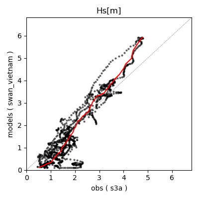
Using the quicklook function again (cco.quicklook(a=True)) will enable three plots this time, a time series plot (ts=True), a map plot (m=True), and a scatter plot (sc=True).
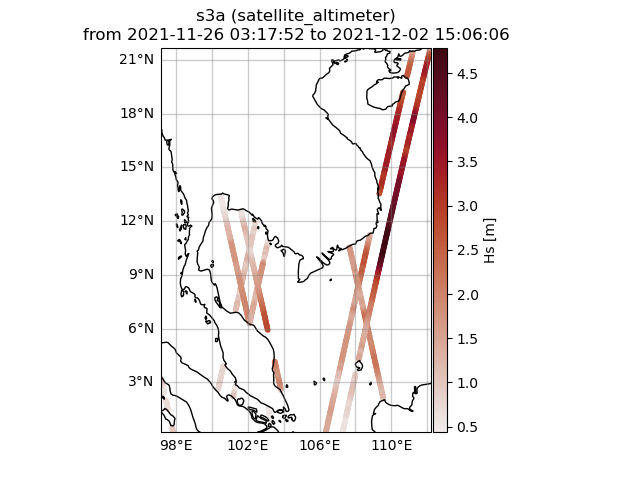
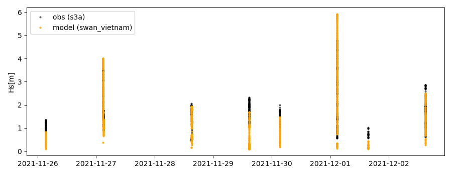
6. Validate the collocated time series
Having collocated a quick validation can be performed using the validationmod. validation_specs.yaml can be adjusted.
>>> val_dict = cco.validate_collocated_values()

# ---
Validation stats
# ---
Correlation Coefficient: 0.93
Mean Absolute Difference: 0.51
Root Mean Squared Difference: 0.66
Normalized Root Mean Squared Difference: 0.29
Debiased Root Mean Squared Difference: 0.64
Bias: -0.17
Normalized Bias: -0.08
Scatter Index: 34.77
Model Activity Ratio: 1.41
Mean of Model: 1.85
Mean of Observations: 2.01
Number of Collocated Values: 1277
The entire validation dictionary will then be in val_dict.