Vietnam Validation Workshop 2021
Note
The codes used for this workshop are from an older version of wavy. It can be adapted with the newest version of the package, however you can still find the version used for this workshop on github.
The following examples are tailored to the 3. wavy Vietnam Validation Workshop 2021.
1. wavy config files
For this work shop you will need the following config files:
collocation_specs.yaml.default  region_specs.yaml.default
satellite_specs.yaml.default    quicklook_specs.yaml.default
model_specs.yaml.default        variable_info.yaml.default
wavy browses the directory structure as follows:
check if env ‘WAVY_CONFIG’ is set or specified in .env
check if a config folder exists using xdg
fall back on default files within the package
We will start off copying the default config files listed above to a directory of your choice. Then remove the “.default” extension. For simplicity, let’s assume that you have your custom config files in ~/wavy/config/.
The main changes that will occur in this workshop are:
adjusting the path
adding your model
2. download L3 satellite altimetry data
L3 satellite data is obtained from Copernicus with the product identifier WAVE_GLO_WAV_L3_SWH_NRT_OBSERVATIONS_014_001. User credentials are required for this task. So before you can start you have to get a Copernicus account (free of costs). Prepare access to Copernicus products. Enter your account credentials into the .netrc-file. Your .netrc should look something like:
machine nrt.cmems-du.eu login {USER} password {PASSWORD}
Prepare your wavy environment with providing the directories for satellite data and model data. There are multiple config files but we only need to worry about a few for now. Explore the config file for satellites like this:
$ cd ~/wavy/config
$ vim satellite_specs.yaml
Add your path for satellite data here under cmems
cmems_L3:
   dst:
      path_template: /home/patrikb/tmp_altimeter/L3/mission
You can proceed now and download L3 data using the wavyDownload.py script:
$ cd ~/wavy/apps/standalone
To get help check …
$ ./wavyDownload.py -h
… then download some satellite altimeter data:
$ ./wavyDownload.py -sat s3a -sd 2020110100 -ed 2020111000 -product cmems_L3 -nproc 4
You can find the downloaded files in your chosen download directory.
3. download L2P and L3 CCI multi-mission satellite altimetry data
Similarily one can download L2P and L3 multi-mission altimetry data from the CEDA Climate Change Initiative. This spans a long time period from 1991 to 2018 and enables climate related research and wave model hindcast validation. Retrieving this data under https://data.ceda.ac.uk/neodc/esacci/sea_state/data/v1.1_release/{l2p/l3} requires a user account for the CEDA archive at: https://archive.ceda.ac.uk/. This account is free!
In your .netrc you need to add:
machine ftp.ceda.ac.uk login {USER} password {PASSWORD}
For instance for Jason-3 L2P:
$ ./wavyDownload.py -sat j3 -sd 2017112000 -ed 2017112100 -product cci_L2P -nproc 4
Or for instance for a multi-mission L3 file:
$ ./wavyDownload.py -sat multi -sd 2017112000 -ed 2017112100 -product cci_L3
4. read satellite data
Once the satellite data is downloaded one can access and read the data for further use with wavy or other software.
L3 data from cmems
In python L3 data can be read by importing the satellite_class, choosing a region of interest, the variable of interest (Hs or U), the satellite mission, which product should be used, and whether a time window should be used as well as a start and possibly an end date. This could look like:
>>> from wavy.satmod import satellite_class as sc
>>> region = 'NorwegianSea'
>>> varalias = 'Hs' # default
>>> mission = 's3a' # default
>>> product = 'cmems_L3' # default
>>> twin = 30 # default
>>> sd = "2020-11-1" # can also be datetime object
>>> ed = "2020-11-10" # not necessary if twin is specified
>>> sco = sc(sdate=sd,edate=ed,region=region)
This would result in a satellite_class object and the following output message:
>>> sco = sc(sdate=sd,edate=ed,region=region)
# -----
### Initializing satellite_class object ###

Parsing date
Translate to datetime
Parsing date
Translate to datetime
Requested time frame: 2020-11-01 00:00:00 - 2020-11-02 00:00:00
Chosen time window is: 30 min
No download initialized, checking local files

 ## Find files ...
path_local is None -> checking config file
/home/patrikb/tmp_altimeter/L3/s3a/2020/10
/home/patrikb/tmp_altimeter/L3/s3a/2020/11
26 valid files found

 ## Read files ...
Get filevarname for
stdvarname: sea_surface_wave_significant_height
varalias: Hs
!!! standard_name:  sea_surface_wave_significant_height  is not unique !!!
The following variables have the same standard_name:
 ['VAVH', 'VAVH_UNFILTERED']
Searching *_specs.yaml config file for definition
Variable defined in *_specs.yaml is:
Hs = VAVH
100%|███████████████████████████████████████████| 26/26 [00:00<00:00, 91.45it/s]
Concatenate ...
... done concatenating
Total:  46661  footprints found
Apply region mask
Specified region: NorwegianSea
 --> Bounded by polygon:
lons: [5.1, -0.8, -6.6, -9.6, -8.6, -7.5, 1.7, 8.5, 7.2, 16.8, 18.7, 22.6, 18.4, 14.7, 11.7, 5.1]
lats: [62.1, 62.3, 63.2, 64.7, 68.5, 71.1, 72.6, 74.0, 76.9, 76.3, 74.5, 70.2, 68.3, 66.0, 64.1, 62.1]
Values found for chosen region and time frame.
Region mask applied
For chosen region and time:  351 footprints found

## Summary:
Time used for retrieving satellite data: 0.34 seconds
Satellite object initialized including 351 footprints.
# -----
Investigating the satellite_object you will find something like:
>>> sco.
sco.edate             sco.product           sco.units
sco.get_item_child(   sco.provider          sco.varalias
sco.get_item_parent(  sco.quicklook(        sco.varname
sco.mission           sco.region            sco.vars
sco.obstype           sco.sdate             sco.write_to_nc(
sco.path_local        sco.stdvarname
sco.processing_level  sco.twin
With the retrieved variables in sa_obj.vars:
>>> sco.vars.keys()
dict_keys(['sea_surface_wave_significant_height', 'time', 'time_unit', 'latitude', 'longitude', 'datetime', 'meta'])
Using the quicklook fct you can quickly visualize the data you have retrieved:
>>> sco.quicklook(ts=True) # for time series
>>> sco.quicklook(m=True) # for a map
5. access/read model data
Model output can be accessed and read using the modelmod module. The modelmod config file model_specs.yaml needs adjustments if you want to include a model that is not present as default. Given that the model output file you would like to read follows the cf-conventions and standard_names are unique, the minimum information you have to provide are usually:
modelname:
    path_template:
    file_template:
    init_times: []
    init_step:
Often there are ambiguities due to the multiple usage of standard_names. Any such problem can be solved here in the config-file by adding the specified variable name like:
vardef:
    Hs: VHM0
    time: time
    lons: lon
    lats: lat
The variable aliases (left hand side) need to be specified in the variable_info.yaml. Basic variables are already defined. All specs listed here are also used when wavy writes the retrieved values to netcdf.
>>> from wavy.modelmod import model_class as mc
>>> model = 'mwam4' # default
>>> varalias = 'Hs' # default
>>> sd = "2020-11-1"
>>> ed = "2020-11-2"
>>> mco = mc(sdate=sd) # one time slice
>>> mco_p = mc(sdate=sd,edate=ed) # time period
>>> mco_lt = mc(sdate=sd,leadtime=12) # time slice with lead time
Whenever the keyword “leadtime” is None, a best estimate is assumed and retrieved. The output will be something like:
>>> mco = mc(sdate=sd)

>>> mco.
mco.edate             mco.leadtime          mco.units
mco.fc_date           mco.model             mco.varalias
mco.filestr           mco.quicklook(        mco.varname
mco.get_item_child(   mco.sdate             mco.vars
mco.get_item_parent(  mco.stdvarname

>>> mco.vars.keys()
dict_keys(['longitude', 'latitude', 'time', 'datetime', 'time_unit', 'sea_surface_wave_significant_height', 'meta', 'leadtime'])
For the modelclass objects a quicklook fct exists to depict a certain time step of what you loaded:
>>> mco.quicklook() # for a map
Note
Even though it is possible to access a time period, wavy is not yet optimized to do so and the process will be slow. The reason, being the ambiguous use of lead times, will be improved in future versions.
6. collocating model and observations
One of the main focus of wavy is to ease the collocation of observations and numerical wave models for the purpose of model validation. For this purpose there is the config-file collocation_specs.yaml where you can specify the name and path for the collocation file to be dumped if you wish to save them.
Collocation of satellite and wave model
>>> from wavy.satmod import satellite_class as sc
>>> from wavy.collocmod import collocation_class as cc

>>> model = 'mwam4' # default
>>> mission = 's3a' # default
>>> varalias = 'Hs' # default
>>> sd = "2020-11-1 12"
>>> sco = sc(sdate=sd,region=model,mission=mission,varalias=varalias)
>>> cco = cc(model=model,obs_obj_in=sco,distlim=6,date_incr=1)

>>> # plotting
>>> import matplotlib.pyplot as plt
>>> fig = plt.figure(figsize=(9,3.5))
>>> ax = fig.add_subplot(111)
>>> ax.plot(cco.vars['datetime'],cco.vars['obs_values'],color='gray',marker='o',linestyle='None',alpha=.4,label='obs')
>>> ax.plot(cco.vars['datetime'],cco.vars['model_values'],'b.',label='model',lw=2)
>>> plt.legend(loc='upper left')
>>> plt.ylabel('Hs [m]')
>>> plt.show()
This can also be done for a time period:
>>> sd = "2020-11-1"
>>> ed = "2020-11-2"
>>> sco = sc(sdate=sd,edate=ed,region=model,mission=mission,varalias=varalias)
>>> cco = cc(model=model,obs_obj_in=sco,distlim=6,date_incr=1)
For the collocation class object there is also a quicklook fct implemented which allows to view both the time series and a map as for the satellite class object:
>>> cco.quicklook(ts=True)
>>> cco.quicklook(m=True)
7. dump collocation ts to a netcdf file
The collocation results can now be dumped to a netcdf file. The path and filename can be entered as keywords but also predefined config settings can be used from collocation_specs.yaml:
>>> cco.write_to_nc()
8. validate the collocated time series
Having collocated a quick validation can be performed using the validationmod. validation_specs.yaml can be adjusted.
>>> val_dict = cco.validate_collocated_values()

# ---
Validation stats
# ---
Correlation Coefficient: 0.98
Mean Absolute Difference: 0.38
Root Mean Squared Difference: 0.53
Normalized Root Mean Squared Difference: 0.13
Debiased Root Mean Squared Difference: 0.50
Bias: -0.16
Normalized Bias: -0.05
Scatter Index: 16.93
Mean of Model: 2.97
Mean of Observations: 3.14
Number of Collocated Values: 2217
The entire validation dictionary will then be in val_dict.
9. quick look examples
The script “wavyQuick.py” is designed to provide quick and easy access to information regarding satellite coverage and basic validation. Checkout the help:
$ cd ~/wavy/apps/standalone
$ ./wavyQuick.py -h
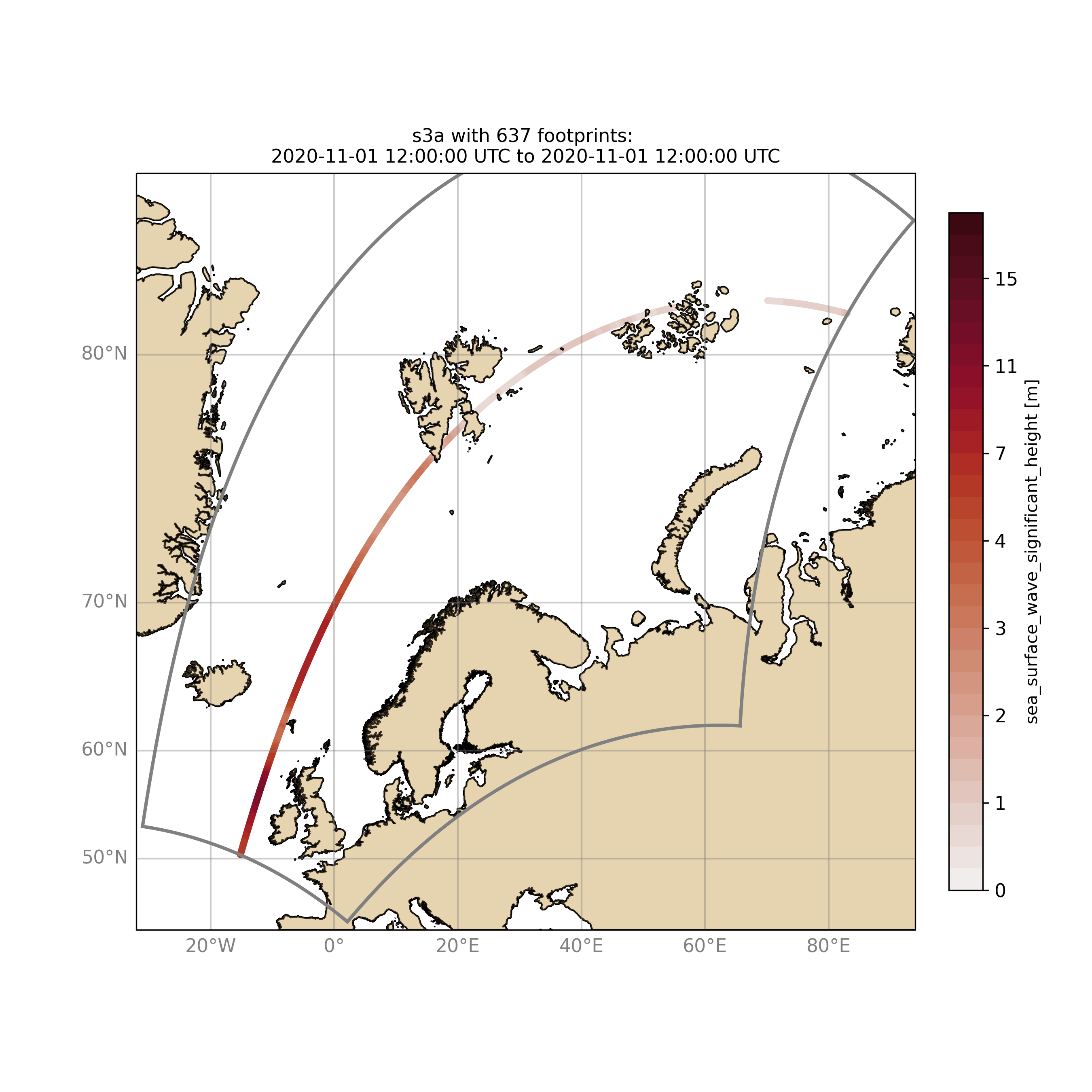
Browsing for satellite data of a given satellite mission and show footprints on map for a given time step and region:
For a model domain, here mwam4
$ ./wavyQuick.py -sat s3a -reg mwam4 -sd 2020110112 --show
or for a user-defined polygon
$ ./wavyQuick.py -sat s3a -reg NorwegianSea -sd 2020110112 --show
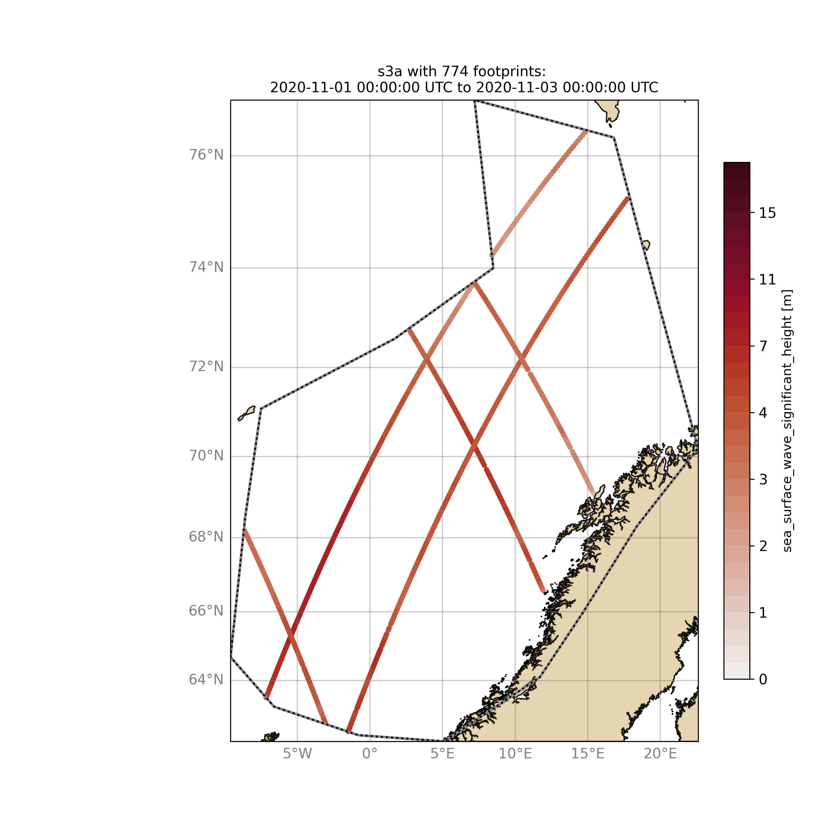
Browsing for satellite data and show footprints on map for time period would be the same approach simply adding an ending date:
$ ./wavyQuick.py -sat s3a -reg NorwegianSea -sd 2020110100 -ed 2020110300 --show
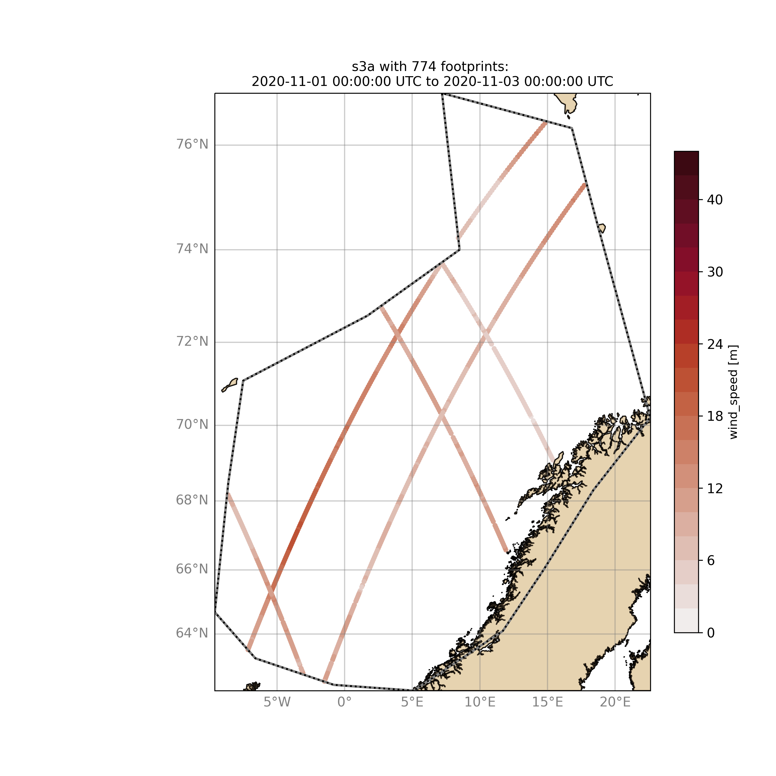
The same could be done choosing 10m wind speed instead of significant wave height:
$ ./wavyQuick.py -var U -sat s3a -reg NorwegianSea -sd 2020110100 -ed 2020110300 --show
The -sat argument can also be a list of satellites (adding the -l argument) or simply all available satellites:
$ ./wavyQuick.py -sat list -l s3a,s3b,al -mod mwam4 -reg mwam4 -sd 2020110112 -lt 30 -twin 30 --col --show
$ ./wavyQuick.py -sat all -mod mwam4 -reg mwam4 -sd 2020110112 -lt 30 -twin 30 --col --show
Now, dump the satellite data to a netcdf-file for later use:
$ ./wavyQuick.py -sat s3a -reg mwam4 -sd 2020110100 -ed 2020110300 -dump /home/patrikb/tmp_altimeter/quickdump/test.nc
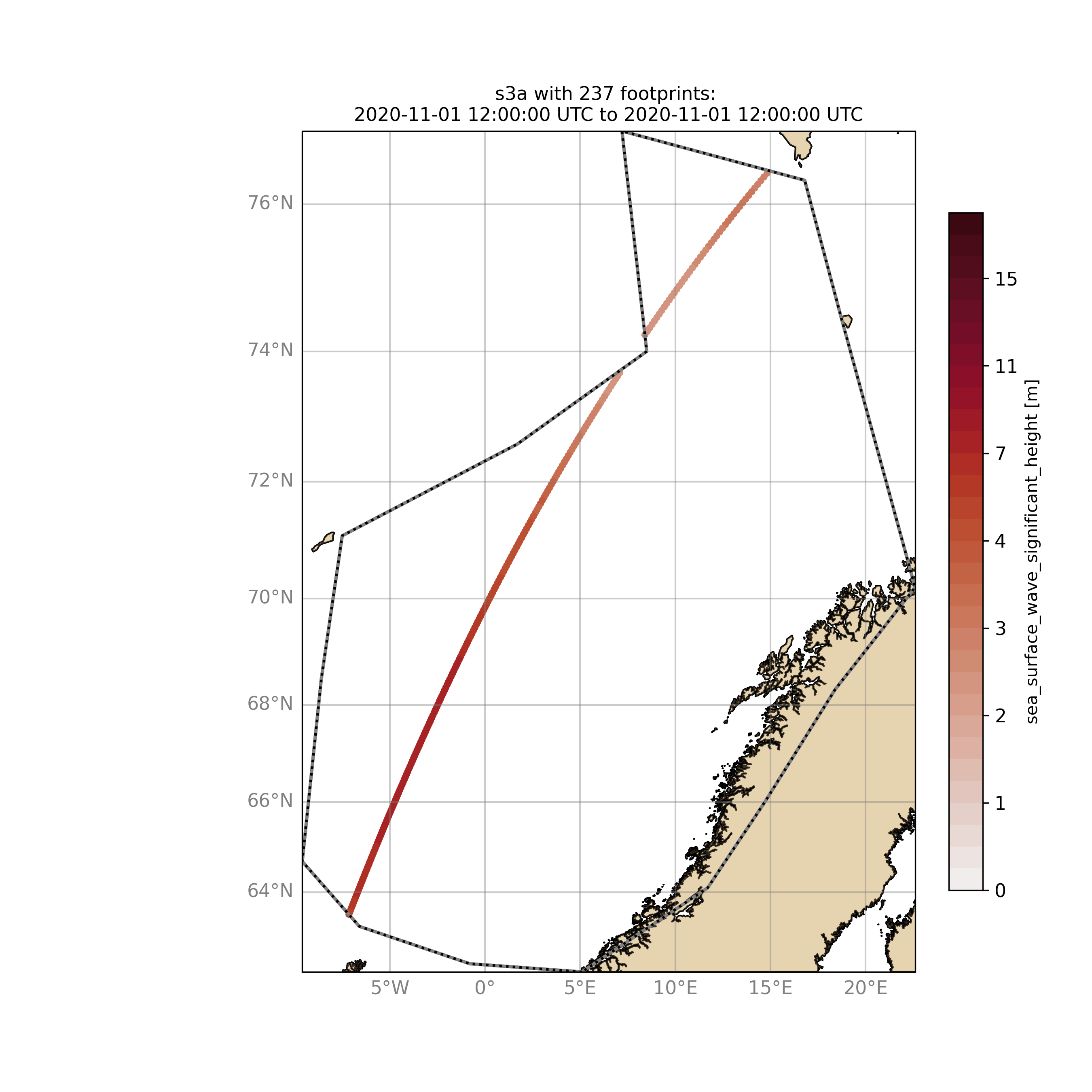
Browse for satellite data, collocate with wave model output and show footprints and model output for one time step and a given lead time (-lt 0) and time constraint (-twin 30):
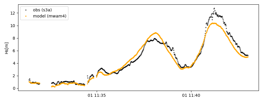
$ ./wavyQuick.py -sat s3a -reg NorwegianSea -mod mwam4 -sd 2020110112 -lt 0 -twin 30 --col --show
This results in a validation summary based on the collocated values:
# ---
Validation stats
# ---
Correlation Coefficient: 0.95
Mean Absolute Difference: 0.62
Root Mean Squared Difference: 0.70
Normalized Root Mean Squared Difference: 0.13
Debiased Root Mean Squared Difference: 0.67
Bias: 0.22
Normalized Bias: 0.04
Scatter Index: 12.71
Mean of Model: 5.26
Mean of Observations: 5.04
Number of Collocated Values: 237
And of course the figure:

10. Vietnam examples
Add model
On order to gather satellite data for your region you need to either specify a region in region_specs.yaml or add your model to model_specs.yaml. For the exercises we will do the latter.
Open your model_specs.yaml file and add:
swan_vietnam:
    vardef:
        Hs: hs
        time: time
        lons: longitude
        lats: latitude
    path_template: "/path/to/your/files/"
    file_template: "SWAN%Y%m%d%H.nc"
    init_times: [0,12]
    init_step: 12
    date_incr: 3
    grid_date: 2021-11-26 00:00:00
    proj4: "+proj=longlat +a=6367470 +e=0 +no_defs"

ecwam_vietnam:
    vardef:
        Hs: significant_wave_height
        time: time
        lons: longitude
        lats: latitude
    path_template: "/path/to/your/files/"
    file_template: "vietnam_wave_%Y%m%d_%H.nc"
    init_times: [0,12]
    init_step: 12
    date_incr: 3
    proj4: "+proj=longlat +a=6367470 +e=0 +no_defs"
    grid_date: 2021-11-26 00:00:00

ecifs_vietnam:
    vardef:
        ux: u10m
        vy: v10m
        time: time
        lons: lon
        lats: lat
    path_template: "/path/to/your/files/"
    file_template: "ECIFS%Y%m%d%H.nc"
    init_times: [0,12]
    init_step: 12
    date_incr: 6
    proj4: "+proj=longlat +a=6367470 +e=0 +no_defs"
    grid_date: 2021-11-26 00:00:00
As path_template I used:
path_template: "/home/patrikb/Documents/Vietnam/%Y/"
Note that date_incr is necessary for wavyQuick.py in order to understand the time steps you have in your model. date_incr is in [h].
Download satellite data
Now, download satellite data for your time period e.g.:
$ cd ~/wavy/apps/standalone
$ ./wavyDownload.py -sat s3a -sd 2021112600 -ed 2021120300 -product cmems_L3 -nproc 4
$ ./wavyDownload.py -sat s3b -sd 2021112600 -ed 2021120300 -product cmems_L3 -nproc 4
$ ./wavyDownload.py -sat c2 -sd 2021112600 -ed 2021120300 -product cmems_L3 -nproc 4
$ ./wavyDownload.py -sat j3 -sd 2021112600 -ed 2021120300 -product cmems_L3 -nproc 4
$ ./wavyDownload.py -sat al -sd 2021112600 -ed 2021120300 -product cmems_L3 -nproc 4
$ ./wavyDownload.py -sat cfo -sd 2021112600 -ed 2021120300 -product cmems_L3 -nproc 4
$ ./wavyDownload.py -sat h2b -sd 2021112600 -ed 2021120300 -product cmems_L3 -nproc 4
Usage in python
Open python and run wavy similar to the example from 4. with your model domain and time period. I tried e.g.:
>>> from wavy.satmod import satellite_class as sc

>>> mission = 'j3'
>>> sd = "2021-11-26"
>>> ed = "2021-12-03"
>>> twin = 30
>>> sco_Hs = sc(sdate=sd,edate=ed,region='swan_vietnam',mission=mission,varalias='Hs',twin=30)
>>> sco_U = sc(sdate=sd,edate=ed,region='ecifs_vietnam',mission=mission,varalias='U',twin=30)

>>> # explore using quicklook fct
>>> sco_Hs.quicklook(ts=True,m=True)
>>> sco_U.quicklook(ts=True,m=True)
Now collocate …
>>> from wavy.collocmod import collocation_class as cc
>>> cco_Hs = cc(model='swan_vietnam',obs_obj_in=sco_Hs,distlim=6,date_incr=3)

>>> # for winds choose correct model and adjust date_incr
>>> cco_U = cc(model='ecifs_vietnam',obs_obj_in=sco_U,distlim=6,date_incr=6)

>>> # explore results
>>> cco_Hs.quicklook(ts=True)
>>> cco_U.quicklook(ts=True)
And validate …
>>> cco_Hs.validate_collocated_values()
>>> cco_U.validate_collocated_values()
Dump collocated files to netcdf …
>>> cco_Hs.write_to_nc() # path from collocation_specs.yaml
>>> cco_Hs.write_to_nc(pathtofile='/path/to/your/file/file.nc')
Dump to validation file is (still) based on single validation dicts that are handed to dumptonc_stats function. This means that e.g. each satellite pass gives one validation number that can be added to one netcdf file. A validation time series file can be established building a loop around.
>>> from wavy.satmod import satellite_class as sc

>>> mission = 'j3'
>>> sd = "2021-11-26"
>>> twin = 30
>>> sco_Hs = sc(sdate=sd,region='swan_vietnam',mission=mission,varalias='Hs',twin=30)

>>> from wavy.collocmod import collocation_class as cc
>>> cco_Hs = cc(model='swan_vietnam',obs_obj_in=sco_Hs,distlim=6,date_incr=3)

>>> from wavy.ncmod import dumptonc_stats
>>> pathtofile = '/home/patrikb/tmp_validation/test.nc'
>>> title = 'validation file'
>>> date = sco_Hs.sdate
>>> time_unit = sco_Hs.vars['time_unit']
>>> validation_dict = cco_Hs.validate_collocated_values()
>>> dumptonc_stats(pathtofile,title,date,time_unit,validation_dict)
The functionality will be expanded in the future such that validation time series can be written based on a collocation object.
wavyQuick use for vietnam model
$ ./wavyQuick.py -sat all -reg ecwam_vietnam -sd 2021112600 -ed 2021120300 -var Hs -twin 30 --show

$ ./wavyQuick.py -sat all -reg ecwam_vietnam -mod ecwam_vietnam -sd 2021112600 -ed 2021120300 -var Hs -twin 30 --col --show