Collocating model output and observations

One of the main focus of wavy is to ease the collocation of observations and numerical wave models for model validation. For this purpose there is a collocation module and a config-file called collocation_specs.yaml where you can specify the name and path for the collocation file to be dumped if you wish to save them.

Collocation of satellite and wave model

>>> from wavy.satmod import satellite_class as sc
>>> from wavy.collocmod import collocation_class as cc

>>> model = 'mwam4' # default
>>> mission = 's3a' # default
>>> varalias = 'Hs' # default
>>> sd = "2020-11-1 12"
>>> sco = sc(sdate=sd)
>>> cco = cc(model=model,obs_obj_in=sco,distlim=6,date_incr=1)

This can also be done for a time period:

>>> sd = "2020-11-1"
>>> ed = "2020-11-5"
>>> sco = sc(sdate=sd,edate=ed,region=model,mission=mission,varalias=varalias)
>>> cco = cc(model=model,obs_obj_in=sco,distlim=6,date_incr=1)

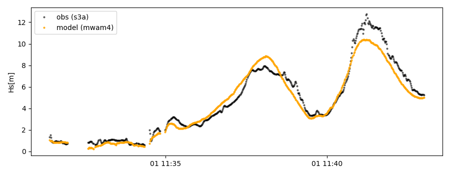
For the collocation class object there is also a quicklook fct implemented which allows to view time series, a scatterplot, and a map as for the satellite class object:

>>> cco.quicklook(ts=True)
>>> cco.quicklook(sc=True)
>>> cco.quicklook(m=True)
>>> cco.quicklook(a=True) # for all plots to be displayed

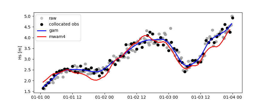
Collocation of in-situ data and wave model

The following example demonstrates the comparison of collocating a raw in-situ time series against a filtered one and may take a few minutes.

>>> # imports
>>> from wavy.insitumod import insitu_class as ic
>>> from wavy.collocmod import collocation_class as cc

>>> # settings
>>> model = 'mwam4' # default
>>> varalias = 'Hs' # default
>>> sd = "2020-1-1 01"
>>> ed = "2020-1-4 00"
>>> nID = 'ekofiskL'
>>> sensor = 'waverider'

>>> # retrievals
>>> ico_gam = ic(nID,sensor,sd,ed,smoother='linearGAM',cleaner='linearGAM',date_incr=1./6.,unique=True,filterData=True)
>>> ico_raw = ic(nID,sensor,sd,ed)

>>> # collocation
>>> cco_gam = cc(model=model,obs_obj_in=ico_gam,distlim=6,date_incr=1)
>>> cco_raw = cc(model=model,obs_obj_in=ico_raw,distlim=6,date_incr=1)

Let’s plot the results:

>>> import matplotlib.pyplot as plt
>>> stdname = ico_raw.stdvarname

>>> fig = plt.figure(figsize=(9,3.5))
>>> ax = fig.add_subplot(111)
>>> ax.plot(ico_raw.vars['datetime'],ico_raw.vars[stdname],color='gray',marker='o',label='raw',linestyle='None',alpha=.4)
>>> ax.plot(cco_raw.vars['datetime'],cco_raw.vars['obs_values'],'ko',label='collocated obs')
>>> ax.plot(ico_gam.vars['datetime'],ico_gam.vars[stdname],'b-',label='gam',lw=2)
>>> ax.plot(cco_gam.vars['datetime'],cco_gam.vars['model_values'],'r-',label='mwam4',lw=2)
>>> plt.legend(loc='upper left')
>>> plt.ylabel('Hs [m]')
>>> plt.show()

Dump collocation ts to a file for later use

The collocation results can be dumped to a pickle or netcdf file. The path and filename can be entered as keywords but also predefined config settings can be used from collocation_specs.yaml:

>>> cco_raw.write_to_nc()
>>> # or
>>> cco_raw.write_to_nc(pathtofile = "/some/random/path/to/file.nc")
>>> # or
>>> cco_raw.write_to_pickle(pathtofile = "/some/random/path/to/file.pkl")