Read in-situ observations (.d22, netcdf/thredds, FROST API)

Currently two data types can be read .d22-files and netcdf-files. Together 4 datasources can be accessed: d22-files, nc-files, thredds-server, FROST API. Edit the insity_specs.yaml file in your config folder and adjust the directories.

read .d22 files

Note

The .d22-files used in these examples and specified here are only available to MET Norway staff. However, The same data will soon be operationally accessible via MET Norway’s FROST API as shown in the examples.

.d22-files can be read in by adjusting d22_var_dicts.yaml config file. Currently, there are wave related variables included. Other variables like wind are about to be included. Another config-file that needs adjustment is the insitu_specs.yaml. There you need to define specs related to the in-situ observation of choice as well as path and filename. A call for the retrieval of an in-situ time series could be like:

>>> from wavy.insitumod import insitu_class as ic
>>> varalias = 'Hs' # default
>>> sd = "2020-01-01"
>>> ed = "2020-01-05"
>>> nID = 'ekofiskL'
>>> sensor = 'waverider'
>>> fifo = "d22" # default
>>> ico = ic(nID, sd, ed, sensor=sensor)

In contrast to the L3 satellite time series, d22 in-situ time series are usually not filtered or underwent rigorous outlier detection. There are various operations that can be performed on the time series. It is in particular interesting to remove double reported values, which is often the case for d22 files. This is done with setting unique=True.

>>> ico = ic(nID, sd, ed, sensor=sensor, unique=True)

make a FROST call

For a FROST call wavy uses MET Norways FROST API v1. A FROST call would be similar compared to the previous example, only the file format needs to be adjusted, here illustrated for the Draugen platform:

>>> nID = 'draugen'
>>> sensor = "MKIIIradar_1"
>>> ico = ic(nID, sd, ed, sensor=sensor, fifo="frost")

read .nc-files

>>> from wavy.insitumod import insitu_class as ic
>>> varalias = 'Hs' # default
>>> sd = "2020-01-01"
>>> ed = "2020-01-05"
>>> nID = 'D_Breisundet_wave'
>>> sensor = 'wavescan'
>>> fifo = "nc" # default for this buoy
>>> ico = ic(nID,sd,ed,sensor=sensor)

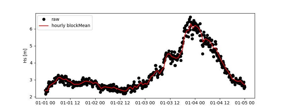
Additionally, outliers can be removed, missing data can be treated, and super-observations can be formed. Below is a example:

>>> # blockMean filter
>>> ico_bm = ic(nID,sd,ed,sensor=sensor,unique=True,priorOp='square',postOp='root',smoother='blockMean',stwin=3,etwin=3,date_incr=1,filterData=True)

Now, let’s check how this could look like:

>>> import matplotlib.pyplot as plt
>>> fig = plt.figure(figsize=(9,3.5))
>>> ax = fig.add_subplot(111)
>>> ax.plot(ico.vars['datetime'],ico.vars[ico.stdvarname],'ko',label='raw')
>>> ax.plot(ico_bm.vars['datetime'],ico_bm.vars[ico.stdvarname],'r-',label='hourly blockMean')
>>> plt.legend(loc='upper left')
>>> plt.ylabel('Hs [m]')
>>> plt.show()

Again, for the insitu class there is also a quicklook fct available:

>>> ico.quicklook()